How to Create a Funnel Chart in Excel 2016
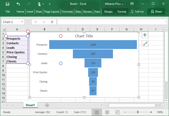
Funnel charts are often used in sales, marketing, and other departments to show data through different stages in a process, such as prospective clients moving through the sales pipeline. A recent update to Office 2016 makes it dead simple to create a funnel chart in Excel.

This new feature is available for Office 365 subscribers.
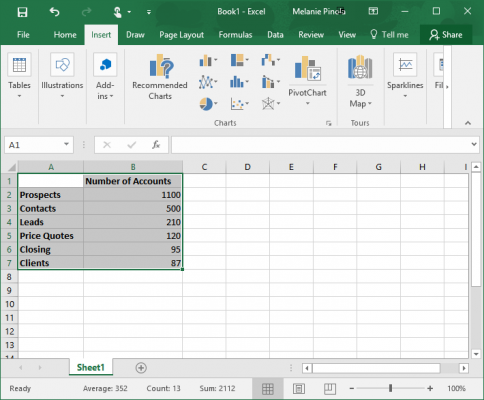
1. Select your data in Excel. It should have a row for each stage of the process and a column for the values.

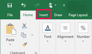
2. Click the Insert tab.

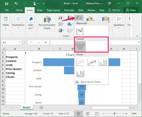
3. Click Insert Waterfall or Stock Chart > Funnel.

Excel will insert the funnel chart for you. Double-click in the chart to format the bars and other design elements of the funnel chart, or go to the Design and Format tabs to quickly customize the chart's appearance.
Microsoft Excel Tips
- Use VLOOKUP in Excel
- Back Up Files Automatically in Excel
- Remove Duplicate Data in Excel
- Create a Waterfall Chart in Excel
- Lock Cells in Excel
- Freeze Rows and Columns in Excel
- Build a Forecast Chart in Excel
- Create a Funnel Chart in Excel
- Make a Treemap in Excel
- Convert Excel Sheets to Google Sheets
- Open Google Sheets in Excel
- Combine Data from Different Cells
- Merge Cells to Span Multiple Columns
- Use AutoFill for Repetitive Data
- Copy and Paste Repetitive Data the Easy Way
- Use Text to Columns
- Draw Diagonal Line in a Cell
- Create a New Shortcut Menu
- Transpose Columns Using Paste Special
Stay in the know with Laptop Mag
Get our in-depth reviews, helpful tips, great deals, and the biggest news stories delivered to your inbox.
