10 Excel Tips You Need to Keep Your Job
In today's dynamic corporate environment, the best way to stay employed is to show the boss that you're indispensable. If you're a knowledge worker of any kind, you probably use Excel a whole lot and so does your boss. While your coworkers may be excellent (or even better than you) at their core jobs, their Excel skills are probably lacking.
If your boss knows that they can turn to you for help with an Excel problem, that makes you the last person they'll want to fire. Here are 10 powerful Excel tips that will make you the most valuable employee in your department.
Remove Duplicate Data
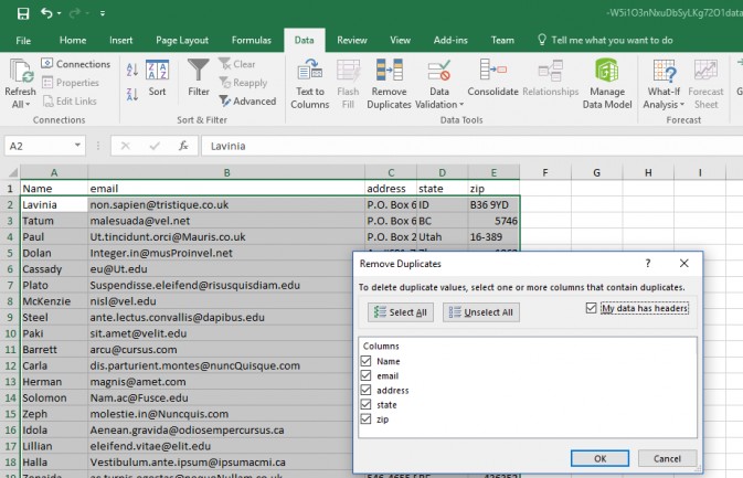
Your boss calls you in, points to her screen and says "this spreadsheet is a mess. Just look at all these duplicate rows. Can you clean this up?" You're going to look like a hero and all you'll need is a few seconds and a couple of clicks. Highlight all of your cells,navigate to the Data tab and click the Remove Duplicates button. You can choose to have the software look only at some columns, but you'll probably want to leave them all checked. Then Click Ok.
Recover Lost Excel Files
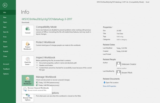
If you have occasion to use this tip to help your boss, you won't just save your job; you'll get a raise. If your boss was working on a spreadsheet and, for some reason, the computer or Excel crashed and she lost all her unsaved work, you can probably get it back. Head over to the File menu in Excel, select theInfotab, click on the Manage Workbook button and then you'll see a menu option which says "Recover Unsaved Workbooks." When you click that menu optoin, you'll see a directory thatcontains any unsaved files.
Use VLOOKUP to Combine Data from Different Sheets
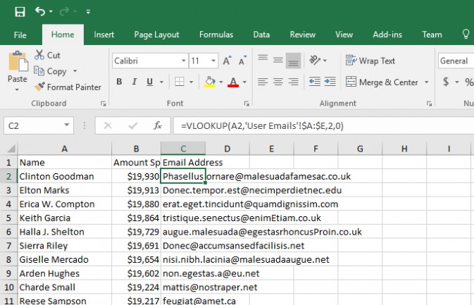
I credit VLOOKUP alone for keeping me employed through the lean years at a previous job. With VLOOKUP, you can match up data from two different spreadsheets, based on having one column of content in common. For example, let's say you have a list of top customers with their names and addresses in one sheet and registered website users with their names and email addresses in the other. You can use VLOOKUP to pair the email addresses from one sheet with the top customers in the other sheet. I often use VLOOKUP to match up a list of most important web articles with the complete list of article page views from Google Analystics. To perform a VLOOKUP, first paste the two spreadsheets that you want into different tabs in the same file (if they aren't already in the same file). Then go to the cell you want the matching result in and enter "=VLOOKUP(" followed by the address of the cell you want to match against. So if the name is the common data point between your two sheets and it's in cell A2, you'll have =VLOOKUP(A2 at this point. Insert a comma and then click through to the tab for the other sheet and highlight all of the cells you wish to search. You'll get a cell range such as 'User Emails'!A:E. Highlight that range and hit F4, which will put dollar signs in front of the cell names so your formula now looks like this:=VLOOKUP(A2,'User Emails'!$A:$E. Now enter a comma followed by the number of columns away from the left side of the sheet you need to go to find the desired data (in this case, an email address). Enter a comma, a zero and a close parens symbol at the end and hit Enter. Your formula will now look like this=VLOOKUP(A2,'User Emails'!$A:$E,2,0).
Use Pivot Tables to Summarize Data
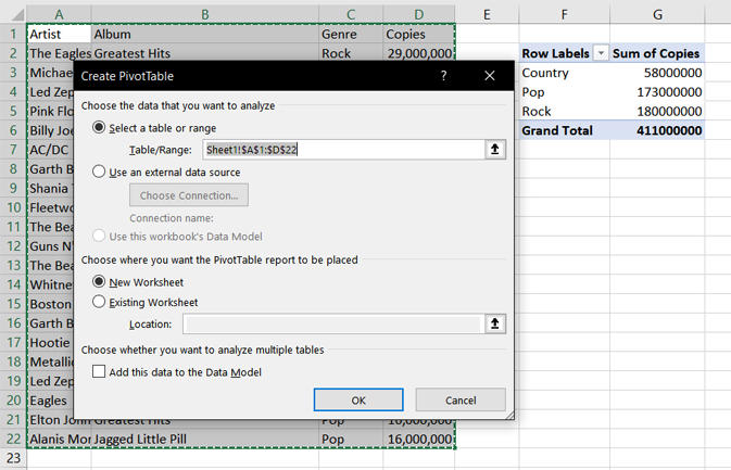
Let's say you've got a spreadsheet full of items -- products for example -- and each one is part of a category. Excel lets you create pivot tables, which show a top-line summary of your data by category. For example, if your spreadsheet were a list of top-selling records with a genre column, a pivot table would give you the sum total of country, pop and rock genres. To create a pivot table, highlight all your data cells and click the PivotTable button on the Insert tab. After you click Ok on the menu box which appears, a blank pivot table appears on a new tab. Check off the names of the columns you want to summarize and your table fills in.
Use Text to Columns to Separate Comma-Delimited Data
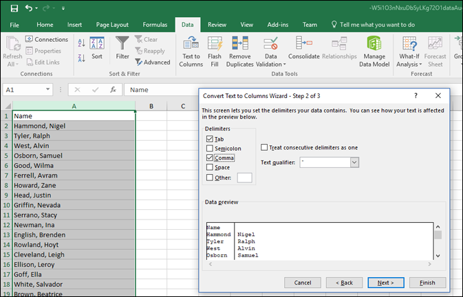
Let's say you or your boss gets a list of names that's written out as "Last Name, First Name." You paste the list into a column on your spreadsheet, but then you realize that you need the first and last names in separate columns. No problem. Just select the column you wish to convert into two columns, navigate to the Data tab at the top of the screen and click the Text-to-Columns button. Then select Delimited and choose "Comma" as the delimiter.If you have a list of items that isn't separated by commas, youcan also choose spaces, semicolons, tabs or any other character as a delimiter.
Stay in the know with Laptop Mag
Get our in-depth reviews, helpful tips, great deals, and the biggest news stories delivered to your inbox.
Draw a Diagonal Line in a Cell
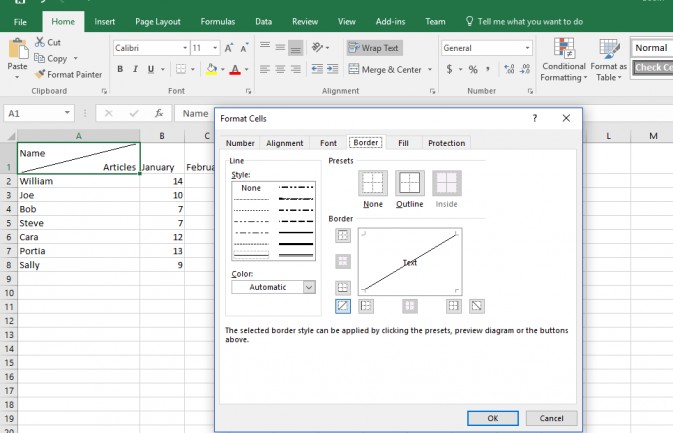
This formatting trick is more showy than practical but it will impress your boss.You can put a diagonal line into a header cell (or any cell) to help you communicate what your data table is all about. For example, let's say we had a column with a list of author names and subsequent columns that contained the number of articles they wrote each month. Rather than putting a title bar above the headers that says "Article Count," you can use the diagonal to show it in the same A1 cell as the "Name" header. To draw a diagonal, right click on the cell (in this case, A1) where you want it to appear and select "Format Cells." Navigate to the Border tab and click the diagonal line box and then click Ok. Type the two pieces of text you wish to separate into your cell and hit Alt + Enter to create at least one line break between them. You'll alsoprobably want to use the space bar to move one of the lines of text over to the right.
Open Google Sheets in Excel
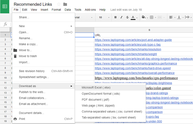
Not every organization standardizes on Excel. What will you do when a partner sends your boss the URL of a Google Sheet and you want to edit that data in Excel? You'll start by telling your boss that you can handle this and that it won't pose a problem. To open a Google Sheet in Excel, you need to download it first. Open the Google spreadsheet in your browser and select "Download As" from the File menu. Then select Microsoft Excel (.xlsx) from the sub menu.
Create an HTML Table in Excel
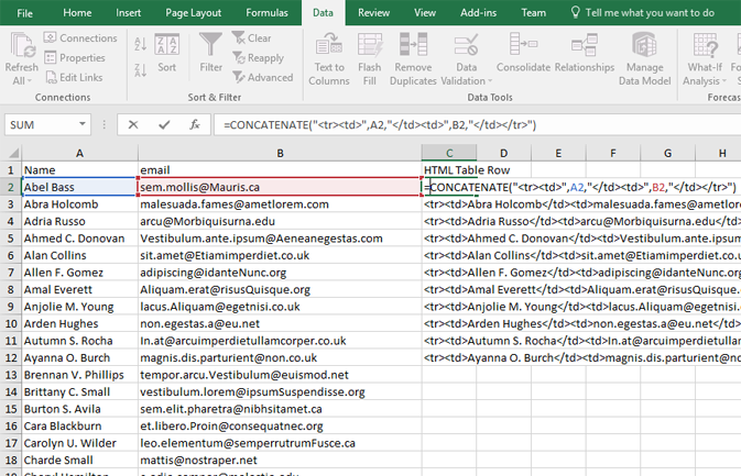
You can save a spreadsheet for web, but if you need to build a specific type ofHTML table, DIV, form or other element, you can use Excel's CONCATENATE formula to build your content. If your job involves publishing content to the web and the company CMS won't let you import data directly from Excel, you'll definitely need this trick. Create a column to the right of your other cells and type =CONCATENATE( into it. You can then combine the relevant HTML for your table with the data from each cell. You just enclose separate each element in the formula with a comma and enclose all of your HTML in quotes. For example, if your A column is a name, and your B column is an address, your HTML column might look like this =CONCATENATE("",A2,"",B2,""). Once you get the CONCATENATE formula right, you can paste it into subsequent rows and the cell addresses will adjust so that the third row will have A3 and B3 and the fourth will have A4 and B4. You can then paste this HTML into your CMS or text editor
Freeze Panes and Make Spreadsheets Easier to Read
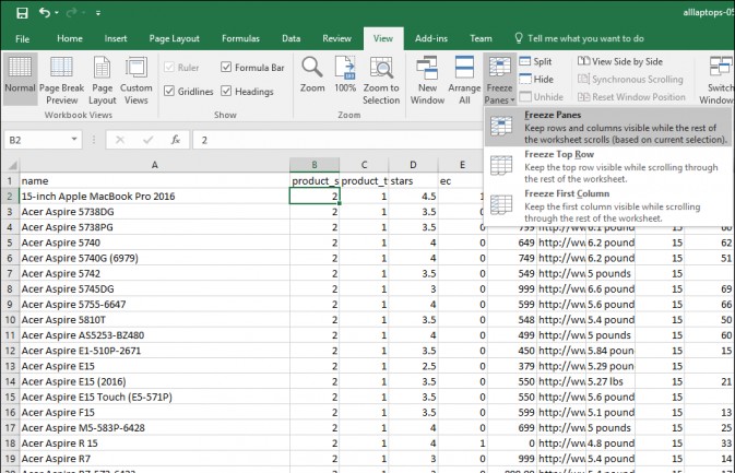
You have a giant spreadsheet with a header row and a very important piece of data -- perhaps it's people's names -- in the left column. However, when you scroll over to Column AA to see the sales figures from two years ago, and move down to row 50 you can no longer see the name and header cells. You're confused and your boss can't understand what you're showing him in your presentation. Freeze some of your columns and rows so that they remain on the screen at all times, even as you scroll around to far-away cells. Just click on the cell that sits one row below the header you wish to keep on screen and one column to the left of the column you want to freeze. In many cases, this will be cell B2. Thennavigate to the View tab, click the Freeze Panesbutton and select "Freeze Panes" from the dropdown menu.

Use Paste Special to Transpose Your Data
It happens all the time. You have a list of items that are going vertically down a column, but you really want them to be laid out horizontally in the same row. Perhaps your boss copied and pasted a vertical list of employees from the company website and wants each to be the header of its own column now. To transpose your data from horizontal to vertical or vertical to horizontal, first highlight and copy the column or row you wish to re-orient. Right click on the cell where you want the data to appear and select Paste Special. Check the transpose box and click Ok.

