How to Freeze Rows and Columns in Excel
Learn how to freeze rows and columns in Excel
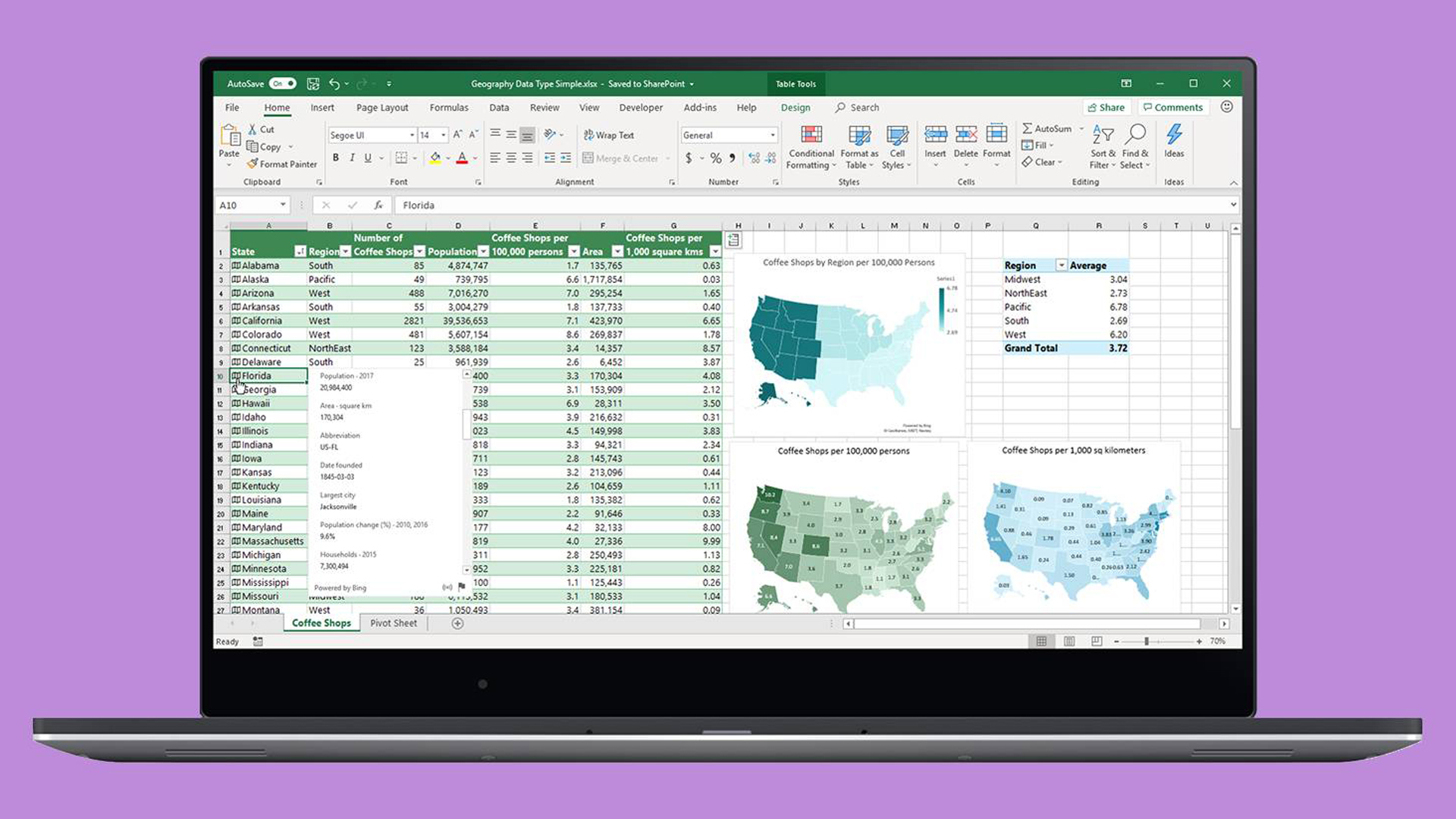
When you're working with a lot of spreadsheet data on your laptop, keeping track of everything can be difficult. It's one thing to compare one or two rows of information when dealing with a small subset of data, but when a dozen rows are involved, things get unwieldy. And we haven't even started talking about columns yet. When your spreadsheets become unmanageable, there's only one solution: freeze the rows and columns.
Freezing rows and columns in Excel makes navigating your spreadsheet much easier. When done correctly, the chosen panes are locked in place; this means those specific rows are always visible, no matter how far you scroll down. More often than not, you'll only freeze a couple of rows or a column, but Excel doesn't limit how many of either you can freeze, which can come in handy for larger sheets.
This how-to works with Microsoft Excel 2016 as well as later versions. However, the this method also works with Google Sheets, OpenOffice and LibreOffice. Ready to get to work? Here's how to freeze rows and columns in Excel:
- More: How to put Windows 10 into Safe Mode
- Here's how to lock cells in Excel and how to recover a deleted or unsaved file in Excel
- This is how to use VLOOKUP in Excel and add additional rows above or below in Excel
How to freeze a row in Excel
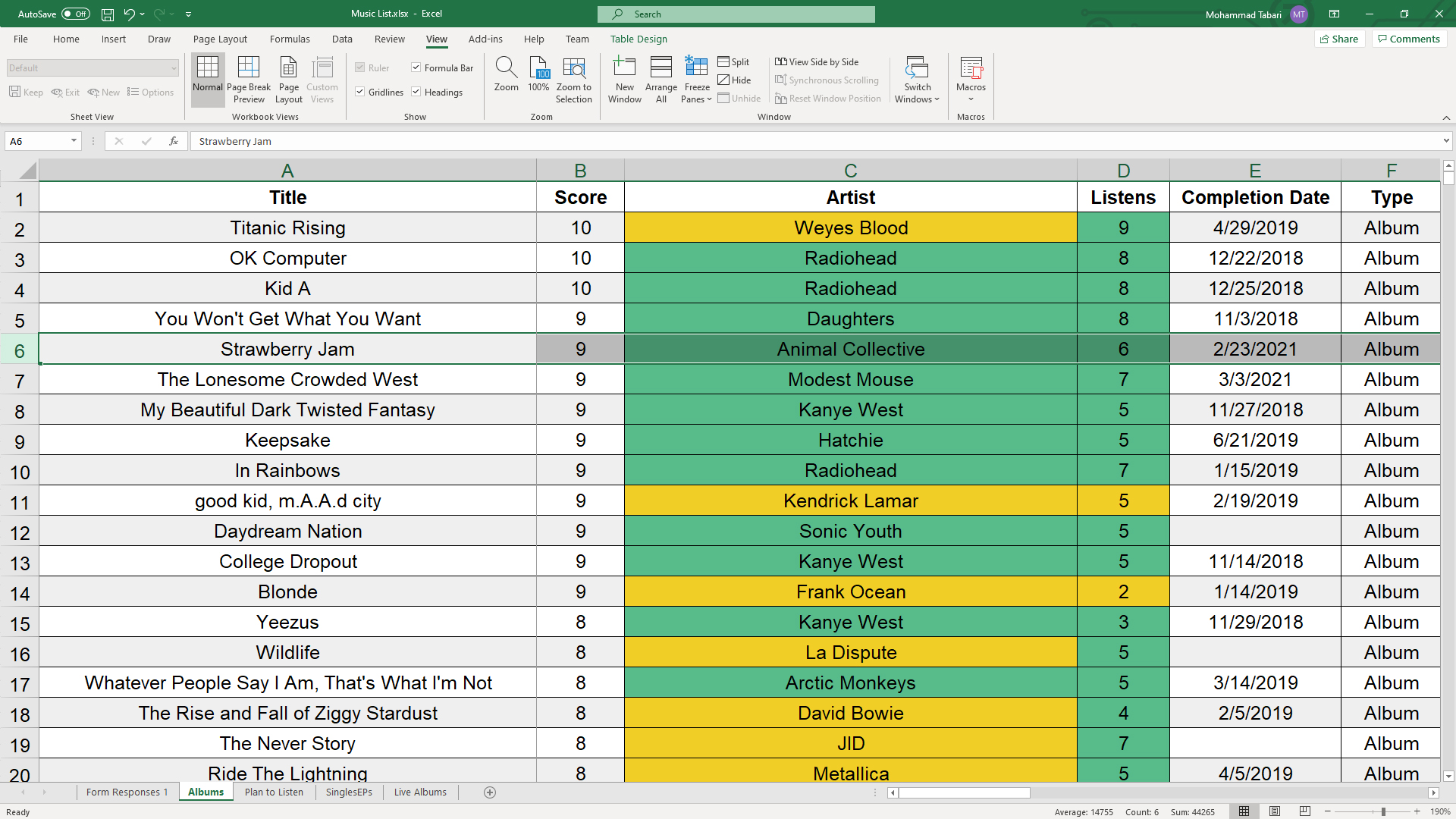
1. Select the row right below the row or rows you want to freeze. If you want to freeze columns, select the cell immediately to the right of the column you want to freeze. In this example, we want to freeze rows 1 to 5, so we've selected row 6.
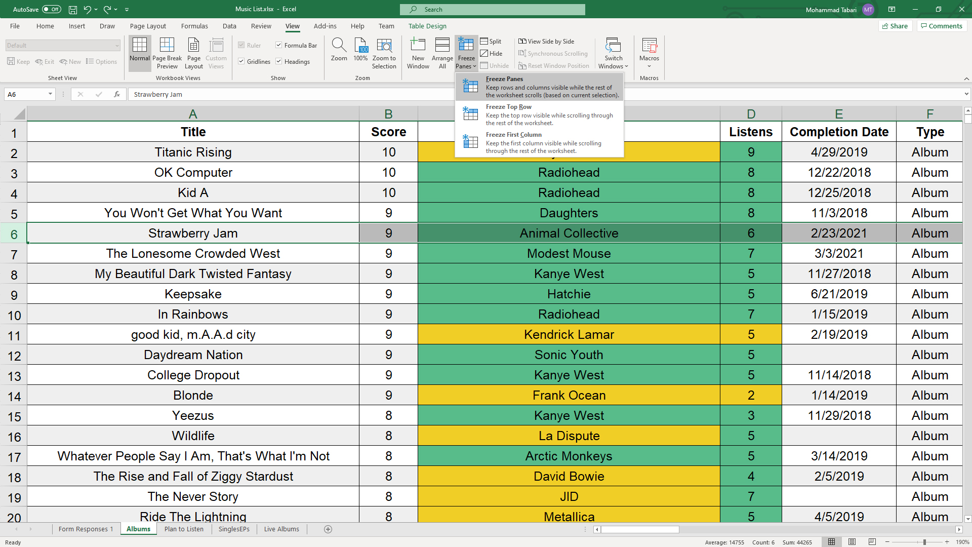
2. Go to the View tab. This is located at the very top, inbetween "Review" and "Add-ins."
3. Select the Freeze Panes option and click "Freeze Panes." This selection can be found in the same place where "New Window" and "Arrange All" are located.
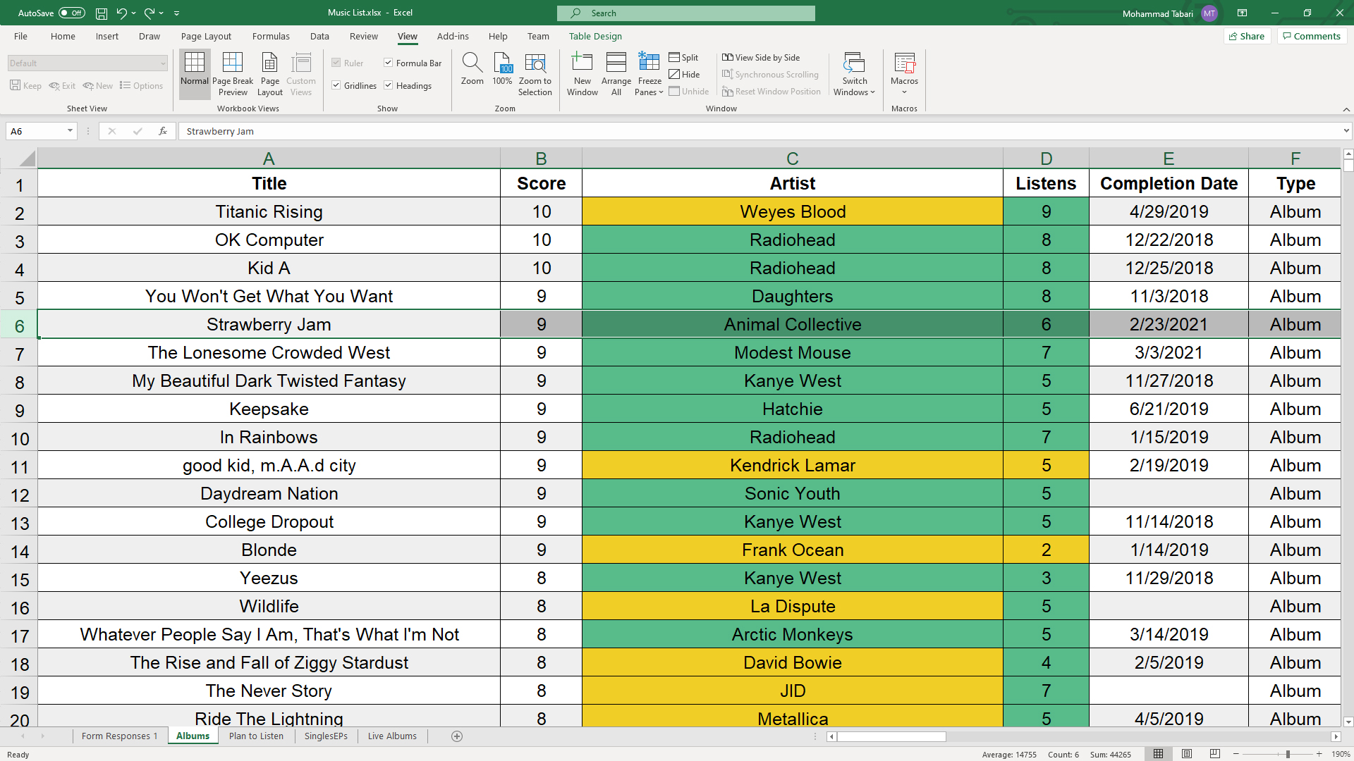
That's all there is to it. As you can see in our example, the frozen rows will stay visible when you scroll down. You can tell where the rows were frozen by the green line dividing the frozen rows and the rows below them.
Get The Snapshot, our free newsletter on the future of computing
Sign up to receive The Snapshot, a free special dispatch from Laptop Mag, in your inbox.
If you want to unfreeze the rows, go back to the Freeze Panes command and choose "Unfreeze Panes".
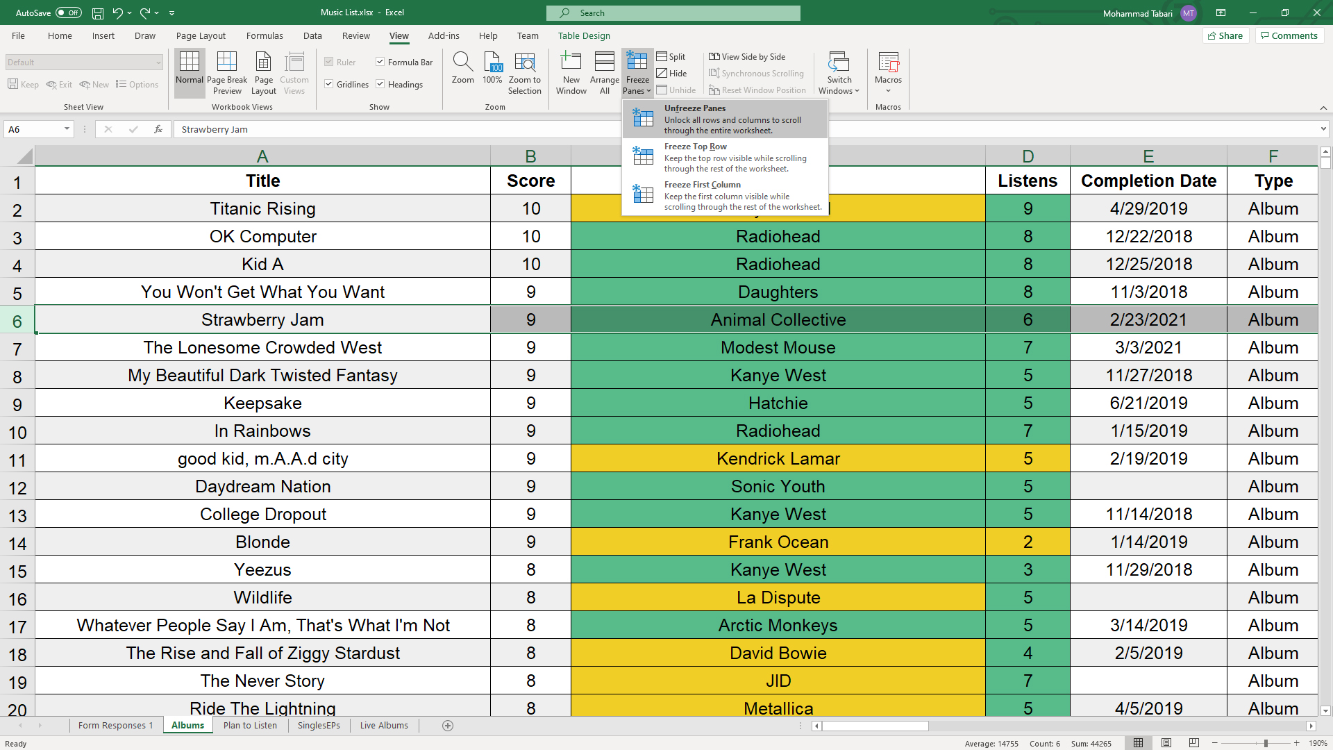
Note that under the Freeze Panes command, you can also choose "Freeze Top Row," which will freeze the top row that's visible (and any others above it) or "Freeze First Column," which will keep the leftmost column visible when you scroll horizontally.
Besides allowing you to compare different rows in a long spreadsheet, the freeze panes feature lets you keep important information, such as table headings, always in view.
Need more Excel tricks? Check out our tutorials on How to Lock Cells in Excel and How to Use VLOOKUP in Excel.
Melanie was a writer at Laptop Mag. She wrote dozens of helpful how-to guides, covering both the software and the hardware side of things. Her work included topics like SSDs, RAM, Apple, Excel, OneDrive, and detailed guides for Windows users. Outside of all her useful advice, Melanie also penned a few reviews for Laptop Mag, including Android emulators that help you run apps on your PC.
