How To Create a Pivot Chart Without a Pivot Table in Excel 2013
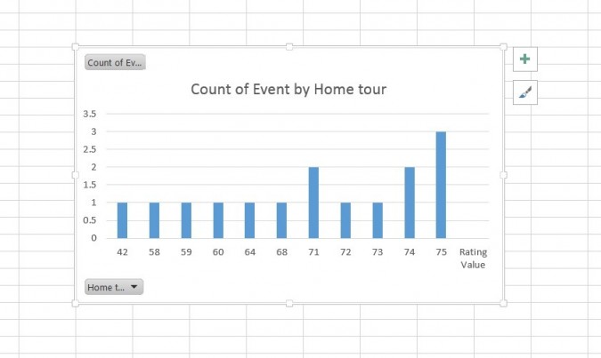
Sometimes you want the flexibility and interactivity of a pivot chart without the hassle of creating a new pivot table. Fortunately, Microsoft Excel 2013 provides exactly that capability. In just a few simple steps, you can create a pivot chart from raw data.
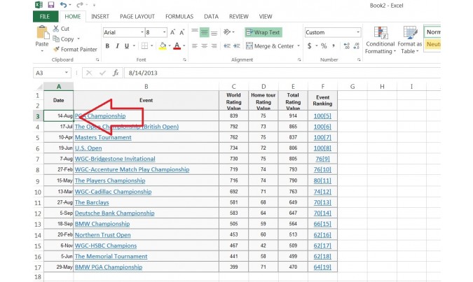
1. Click anywhere inside the data you wish to use for your chart.
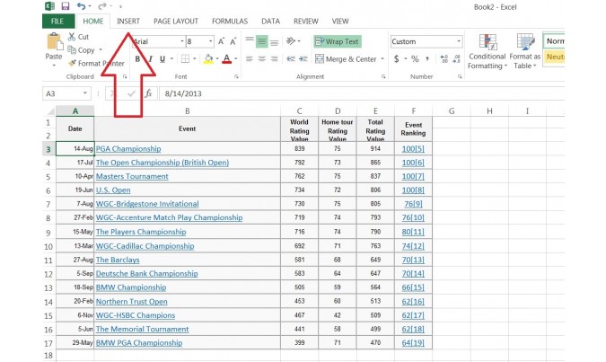
2. Click the "Insert" tab at the top of the screen.
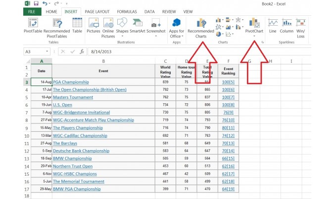
3. Click "Recommended Charts" or "PivotChart" on the Ribbon.
4. Select a Chart with the PivotChart icon in the upper right corner.
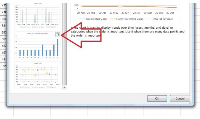
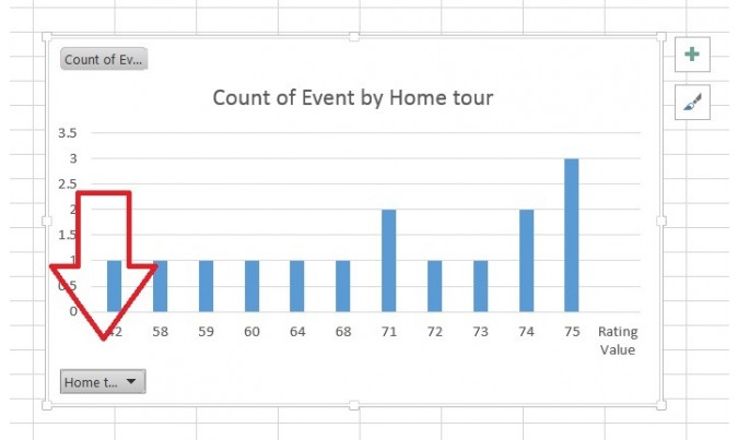
5. Choose filtering options using the interactive controls on the newly created pivot chart.
- 5 Free PC Maintenance Programs Worth Downloading
- 8 Essential Tips for Your New Windows 8 PC
- The Best Free Software for Students
Stay in the know with Laptop Mag
Get our in-depth reviews, helpful tips, great deals, and the biggest news stories delivered to your inbox.
David was a writer at Laptop Mag. His coverage spanned how-to guides, reviews, and product rankings. He reviewed Asus, Lenovo, and Gigabyte laptops; guided readers on how to do various things in Excel, and even how to force quit an app in macOS. Outside of Laptop Mag, his work has appeared on sites such as Tom's Guide and TechRadar.
