How to protect cells, columns, and rows from accidental editing in Excel
Here's how to stop accidental editing in specific parts on your Excel spreadsheet
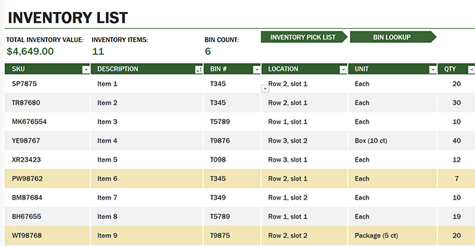
Most people know that you can protect individual rows, columns, or cells in Excel. You can even protect the entire sheet. What they’re not aware of, however, is that you can protect only specific parts of a spreadsheet, parts that are more than a few columns or rows, but not quite the entire workbook.
This level of protection comes in handy when working with multiple users on the same sheet. Now, you can lock the area you’re responsible for and stop worrying that a collaborator will accidentally edit it.
- How to use Microsoft Excel like a pro and how to recover a deleted or unsaved file in Excel
- How to convert Excel spreadsheets to Google Sheets
- How to transpose columns and rows using Paste Special in Excel
How to protect cells, columns, and rows from accidental editing
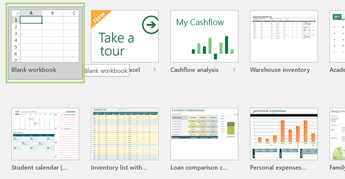
1. Open Excel and select a workbook. For the sake of this tutorial, I’m going to use one of Excel’s default templates.
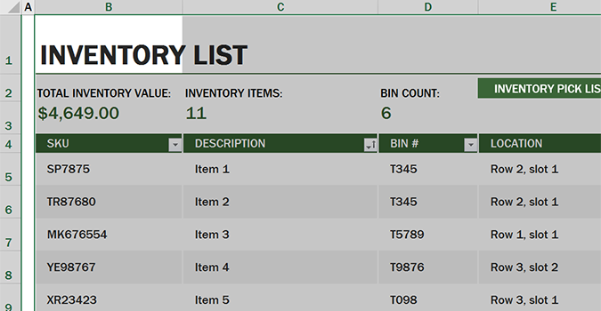
2. First we have to unlock the workbook, which is typically locked (as a whole) by default. To do that, press Ctrl + A to select the entire document.
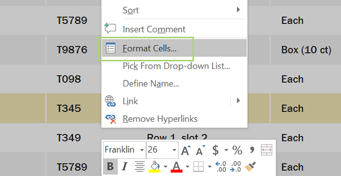
3. Right click and choose Format cells.
4. Under the Protection tab, uncheck Locked. If it’s not checked by default, you’re ready to go. <uncheck.png>
5. Press OK.
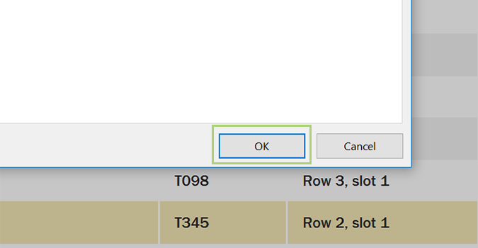
With your workbook now unlocked, we can set about locking specific areas. For the sake of this tutorial, we’re going to pretend we’re responsible for Column B, C, and D.
Stay in the know with Laptop Mag
Get our in-depth reviews, helpful tips, great deals, and the biggest news stories delivered to your inbox.
6. Select the area of the workbook you’d like to protect.
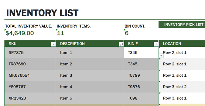
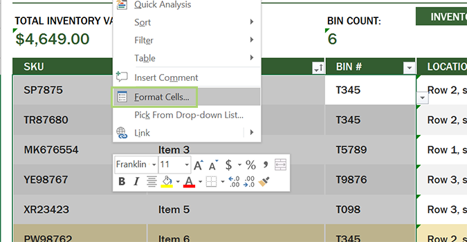
7. Right click and select Format cells. Alternatively, you can use the keyboard shortcut Ctrl + 1.
8. Check Locked and press OK.
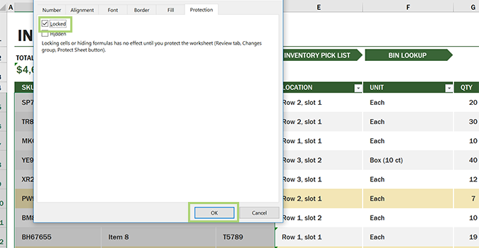
In an Excel workbook, nothing is ever really locked until you protect the sheet. We’re going to do that next.
9. Under the Review tab (in the Ribbon), choose Protect Sheet.
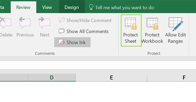
10. Add a password (if desired), and choose what you’d like other users to be able to edit in your protected section. If you’d rather them not touch it at all, uncheck each of the boxes and press OK.
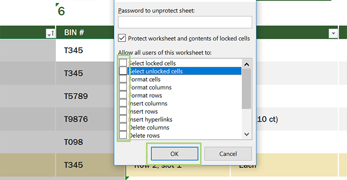
Now, if you try clicking in any of the three columns we protected, nothing happens. Just the way we wanted it.
Bryan covers everything you need to know about Windows, social media, and the internet at large for Laptop Mag. Thanks to his extensive knowledge of operating systems and some of the most popular software out there, Bryan has written hundreds of helpful guides, including tips related to Windows 11 drivers, upgrading to a newer version of the OS, editing in Microsoft Photos, or rearranging pages in Google Docs.
