7 basic Excel functions everyone should know
Excel is powerful, but only if you know how to use it

Sign up to receive The Snapshot, a free special dispatch from Laptop Mag, in your inbox.
You are now subscribed
Your newsletter sign-up was successful
Huge chunks of the world’s data reside in Excel spreadsheets. From finance to health, businesses and institutions the world over still use these spreadsheets to manage, or aid in managing massive operations. For more casual users, Excel spreadsheets can handle everything from meal planning to budgets. It really is the Swiss Army Knife of computer software.
Microsoft Excel is a spreadsheet software with a suite of powerful mathematical, analytical, and visualization tools. Introduced way back in 1987, the software now offers more than 500 functions that can cater to almost any mathematical or analytical needs you have.
It is also available for almost all operating systems, such as Windows, macOS, Ubuntu, Linux, and more. The spreadsheet program is also available on Android and Apple smartphones.
Article continues belowHere are some of the best Excel functions that we believe everyone should know. We will also throw in some samples to help you understand them.
Seven Excel functions you need to learn
SUM
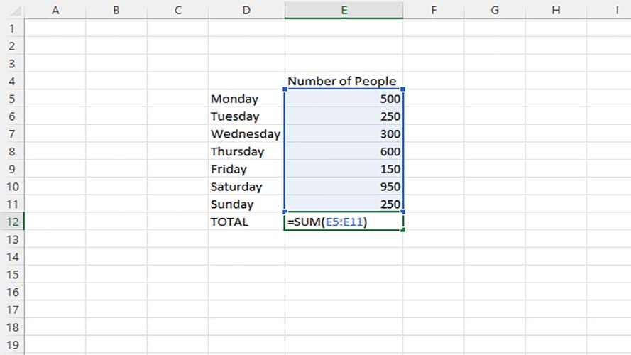
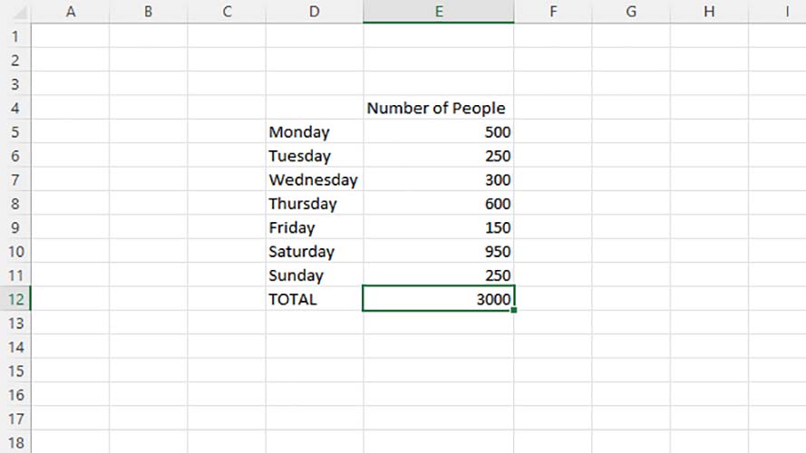
One of the most basic Excel functions, the SUM function, lets you add together a set of numerical data. It is a great substitute for manually choosing each cell then adding an add operation (+) between them. Although very basic, not understanding this function will make it difficult to follow along with some of the more advanced functions below.
Proper Syntax:
=SUM(number1,[number2],...)
Sign up to receive The Snapshot, a free special dispatch from Laptop Mag, in your inbox.
Example:
=SUM(A1, A2, A3)
This formula will tell Excel to get the sum of all numbers inside cells A1, A2, and A3. Note that if any of the values included in the function are non-numerical (e.g., texts), Excel will return a #VALUE! Error.
IF
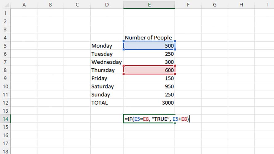
Using the IF function tells Excel to return whether or not the statement provided to it is true or false. It is often used to logically compare data. The function also allows you to set your preferred outcome in case the result of the comparison is true or false.
Proper Syntax:
=IF(logical_test, value_if_true, [value_if_false])
Example:
=IF(A1=A2, “TRUE”, A1+A2)
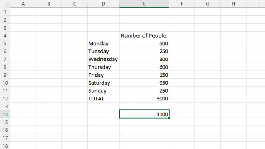
With the formula above, Excel will determine whether or not the value in cells A1 and A2 are logically the same. If the answer is yes, it will return the string “TRUE”. If not, it will return the sum of cells A1 and A2.
CONCATENATE
Concatenate simply stitches together the given values into one whole string of text. If it is given a number or other types of value other than text, it will treat them as text and proceed to combine them accordingly. This formula is very useful when generating long strings of text based on changing variables.
Proper Syntax:
=CONCATENATE(text1, [text2], ...)
Example:
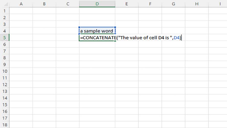
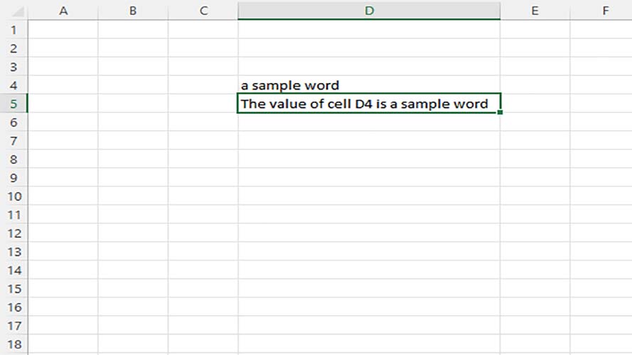
=CONCATENATE(“The value of cell A1 is “, A1)
In the formula above, if A1 has a value of “a sample word”, it will return the text string “The value of cell A1 is a sample word”.
VLOOKUP
Now, we are starting to dive into more complex functions. VLOOKUP is one of the most powerful and useful functions for analyzing data. Its job is to search for a match in the leftmost column of a table array that you provide it, then return the value of the cell in the return column on the same row of the value that matched.
Proper Syntax:
=VLOOKUP (lookup_value, table_array, col_index_num, [range_lookup])
Example:
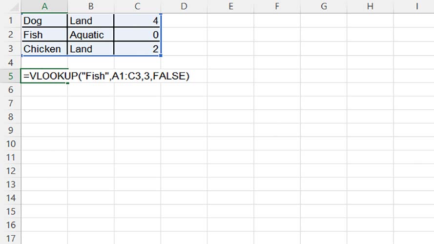
| Row 0 - Cell 0 | A | B | C |
| 1 | Dog | Land | 4 |
| 2 | Fish | Aquatic | 0 |
| 3 | Chicken | Land | 2 |
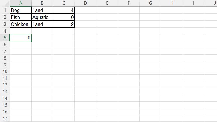
=VLOOKUP (“Fish”, A1:A3, 3, FALSE)
The formula above will process the table array A1:A3. It will search for the word “Fish” on column A, then return the value from column C on the same row as the word “Fish”. Since we specified “FALSE” as the fourth value, the formula will look for an exact match. The expected result of this formula should be 0.
INDEX
Index is another powerful function that users can use for extracting data in a large array of values. Its job is to return a value within an array based on the provided row number and column number.
Proper Syntax:
=INDEX(array, row_num, [column_num])
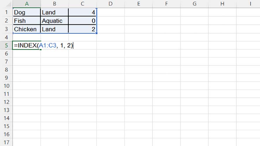
Example:
| Row 0 - Cell 0 | A | B | C |
| 1 | Dog | Land | 4 |
| 2 | Fish | Aquatic | 0 |
| 3 | Chicken | Land | 2 |
=INDEX(A1:A3, 2, 3)
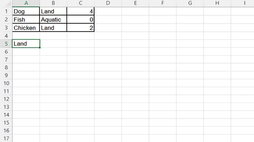
When interpreted, the above tells Excel to search table A1:A3, for the value located at row 2 and column 3. So, the expected result should be Land.
FIND
The FIND function is generally used to process long strings of text. It helps the user find the position of a text within another text. It is case-sensitive, meaning its results are affected by the case of the two texts. It also returns the position of the string that first matches your find text.
Proper Syntax:
=FIND(find_text, within_text, [start_num])
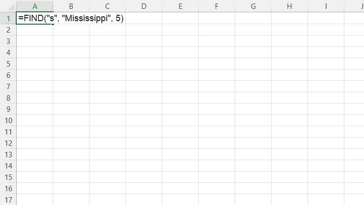
Example:
=FIND(“s”, “Mississippi”, 5)
In the formula above, starting from the fifth character, we will search for the position of “s” from “Mississippi”. The expected result should be 6.
MATCH
Our last must-learn function in excel is MATCH. MATCH is the opposite of INDEX. With INDEX, we specify a row and column position, and Excel tells us the value within that cell. While in MATCH, we look for the position of a value within a given range of cells.
Used together, these two functions provide a similar action as the VLOOKUP function but better as it allows you to search not just the leftmost column. MATCH is not case-sensitive when it comes to texts.
Proper Syntax:
=MATCH(lookup_value, lookup_array, [match_type])
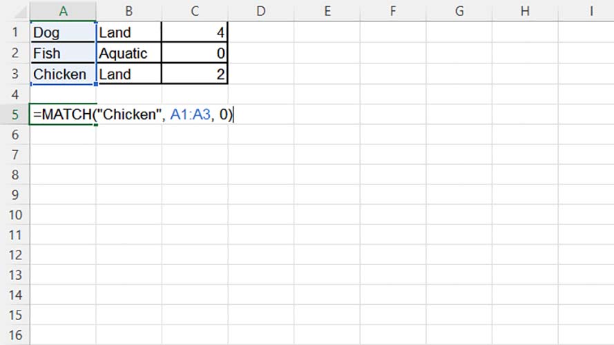
Example:
| Row 0 - Cell 0 | A |
| 1 | Dog |
| 2 | Fish |
| 3 | Chicken |
=MATCH(“Chicken”, A1:A3, 0)
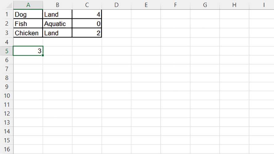
The formula above tells Excel to look for the position of an exact match to “Chicken” from array A1:A3. The expected result should be 3.
