How to use Index Match in Excel
Sift through your Excel data quickly

Knowing how to use Index Match in Excel is one of the most valuable tricks in your productivity software arsenal. Finding specific items in a spreadsheet is easy if it’s small enough. But once you start dealing with data sets that reach hundreds or thousands, complications start to pile up. Luckily, we have several tricks within Microsoft Excel that can help. At the top of this list is Index Match.
Index Match combines two of Microsoft Excel’s best functions. The Index function returns a value from a table or array based on the row and column numbers you provide. The Match function, on the other hand, returns a number that represents the position of a specified value within an array. If you are familiar with how to use VLOOKUP in Excel you can probably already see how powerful this is as unlike VLOOKUP it isn’t limited to searching a single column and it doesn’t dictate your sort order.
The best use for Index Match is to find an item related to another object within the same table. For example, let’s say you have a list of a hundred dogs and their favorite foods. Using Index Match, you can find a specific dog’s favorite food without scrolling up and down your spreadsheet. This is the power of knowing how to use Index Match.
How to use Index Match in Excel
1. In using Index Match, you will use the function template below:
=INDEX(array, MATCH(lookup_value, lookup_array,[match_type]),[column_num])

- array - represents the table or array your data are stored in
- lookup_value - the “independent” value you will reference to find your “dependent” value
- lookup_array - the array of “independent” values where your reference value is included
- [match_type] - allows you to set your Match function to look for an item greater, equal, or less than your reference value.
- [column_num] - an optional value needed if your array has more than one column
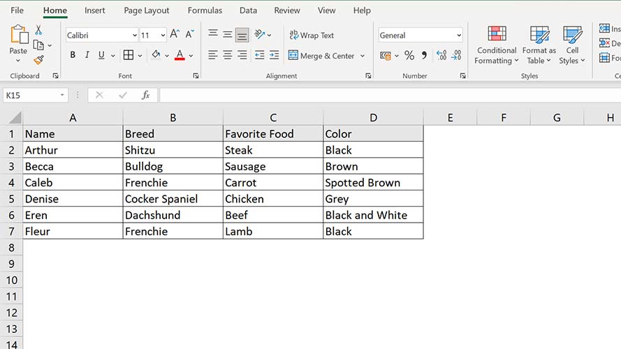
2. We will use the table below as an example. This table lists the dogs in a veterinary clinic. It shows each dog’s name, breed, favorite food, and color.

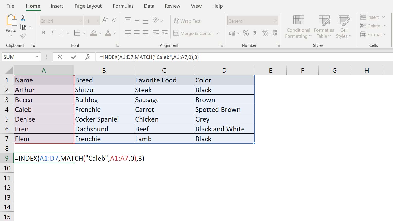
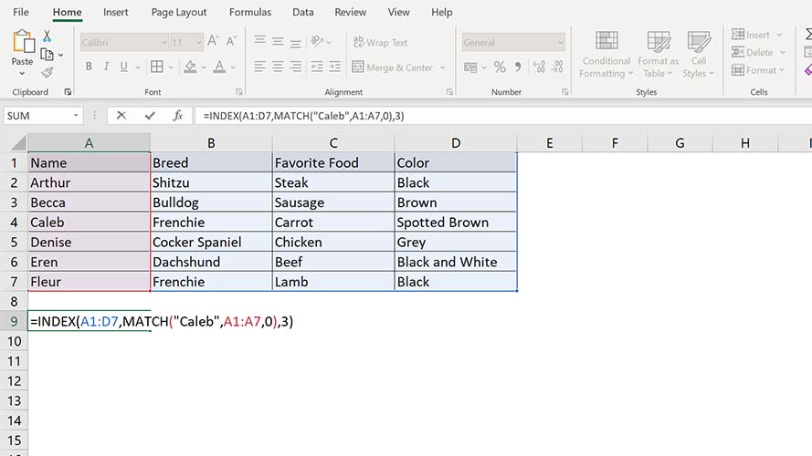
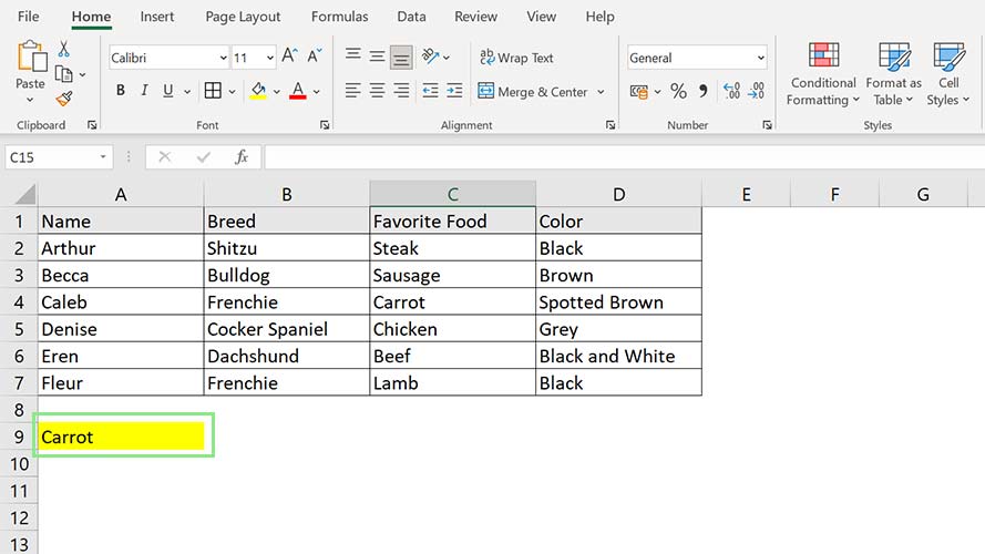
3. If, for example, we want to find Caleb’s favorite food, we will use the function below.
Stay in the know with Laptop Mag
Get our in-depth reviews, helpful tips, great deals, and the biggest news stories delivered to your inbox.
=INDEX(A1:D7, MATCH(“Caleb”, A1:A7,0),3)

- array = A1:D7
- lookup_value = “Caleb”
- lookup_array = A1:D7
- [match_type] = 0 (exact match)
- [column_num] = 3 (food is the third column of the table)
That’s all there is to it, you can try it out yourself and take another step closer to using Excel like a pro. If you want to unlock even more advanced Excel features you should take a look at how to add the Developer tab to Excel.
