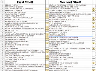
How to Use Google Sheets Conditional Formatting
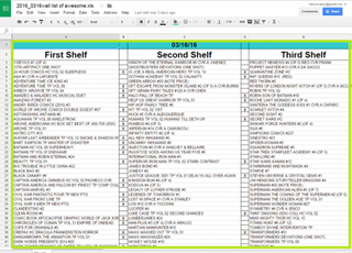
If you're trying to make a large spreadsheet easier to read, you'll likely want to format certain items to highlight what's important for the reader. While you could go in and format each cell by hand, Google Sheets allows you to automate this task with Conditional Formatting Rules.

You can set up a variety of rules for Sheets to obey, including determining whether a cell is empty or not, if it contains a date that is before or after a specific point in time or if it contains text that starts or ends with a particular phrase. Here are our step-by-step instructions for how to use conditional formatting in Google Sheets.
MORE: How to Wrap Text in Google Sheets
1. Select cells you want to apply conditional formatting to.
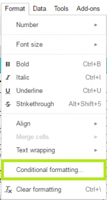
2. Click Format.

3. Select Conditional formatting.
4. Click Cell is not empty.
Stay in the know with Laptop Mag
Get our in-depth reviews, helpful tips, great deals, and the biggest news stories delivered to your inbox.
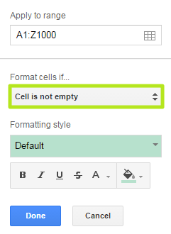
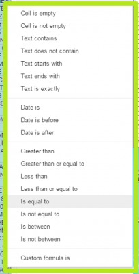
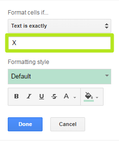
6. Enter the value your condition refers to. If you chose Cell is empty or Cell is not empty, will skip this step.
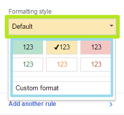
7. Click Default and select a formatting style to apply to the cells.
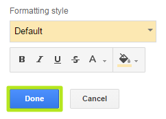
8. Click Done.
Your Google Sheets spreadsheet now follows conditional formatting rules.
